In 2020 the world shut down for a little bit and everyone got new hobbies. COVID was especially nice for me because my classes went online, which is a much easier way to get through your last two semesters of labs as a Microbiology student. The fall of my senior year I had an excess of free time, brain space, and expendable income (thanks to a fruitful summer of running one of the only open restaurants in Arlington, VA). So when some friends reached out to see if I’d be interested in playing World of Warcraft with them I figured it was a convenient way to kill time.

Plot twist: I’ve logged in to that video game every damn week since.

When I first started raiding I was introduced to a website calld “Warcraft Logs”. It’s a massive data analytics dashboard that let’s players link the combat log, a tracking log built into the game that shows every combat-related event that occurs, and analyze time series information to improve their performance. I fell madly in love with the process of looking through the website, analyzing data, and making conclusions. I’ve spent more time pouring through Warcraft Logs than I’ve spent playing the actual game.

I’m telling this story because it’s legitimately the origin of my career in statistics. Had it not been for picking up World of Warcraft as a winter COVID hobby, I wouldn’t have become a statistician.

Ever since I started studying the formal science of statistics I’ve become completely disillusioned to Warcraft Logs (shorthand WCL). The website is an incredible and accessible tool for most people. For true statistical inference though it’s a solid 3/10 product. The best thing about WCL is that it aggregates the data from the combat log— beyond that it’s a bit terrible for my purposes.

For a while now I’ve been wanting to pull data from WCL to develop some real models and metrics that we (the community) can use. Even some of the top groups in the game use ranking percentages, simple summary statistics, and questionable derived quantities to make bulk inference on player performance. The more scientifically minded groups go through player actions line by line to figure out what the players are do. Regardless of method used (beyond testimony from others and video evidence), nobody has ever been able to accurately predict whether a player was going to be capable or a burden. I’d like to change that.

This one is going to be particularly challenging from a ‘data science’ perspective because Warcraft logs .csv files are dirtier than the toilet seats in the singular bathroom at a college nightclub. But this is also a great chance for me to play around with some fun ideas I’ve had for (actually impactful and scientific) research that I’d never be able to test drive otherwise.

If I was laying this out in a book I would title chapter one, “Data Mining Hell”. WCL data is organized generally as:

Overall raid night

— Specific boss fights

---- Pulls (attempts) of the boss fight

------ Individual player data for that attempt

Most people reviewing logs start at the “Pulls” level, which seems like a lot of data but is actually miniscual. Each pull is a sample size of $n=1$ for (typically) 20 players. In order to have a chance at a useful quantity of data I need to grab the data using an API call.

Prior to this, I had no idea how to do an API call. Turns out it’s fucking awful.

I’ll spare the gruesome details on how I performed the API call. Partially out of shame for how it’s likely the worst code I’ve ever written, partially because it’s bad form to reveal the tokens and secrets involved.

The steps make it seem pretty simple though:

1. Download Postman (I’m not doing this with curl, no shot)

2. Set up a client through WCL

3. Use my client ID and secret to get an access token

4. Access a specific guilds log reports

5. Choose a log report

   a. Get every pull of every boss from the report

   b. Organize it by damage taken and done, deaths, and healing done

   c. Shove it all into a JSON file

In this case I chose the guild “All Washed Up”, a US region guild on the server Sargeras. The friends who first introduced me to WCL are raiding in that guild and one of them is doing their analytics by hand. It felt like a good opportunity to test drive some of my ideas and have someone ready to proof check.

I know my query was bad because the data is still horrendously messy. That said I’m confident it’s going to take less time to clean messy JSON files than it would to learn to write better queries. Here goes nothing.

I’ve never worked with unstructured data before. As it turns out it’s not fun. Like I said, the data is shoved into one monolithic JSON file. The file contains 32 separate pulls from two bosses so for each player I should have $n=32$. I converted the JSON into a huge nested list using jsonlite in R:

1
library(jsonlite)
2
j = fromJSON('data/AWU_log1.json', simplifyVector = FALSE)

The list is organized by damage taken, damage done, deaths, and healing done, for each pull. Since they’re in that specific order I decided to separate them with a set of simple loops. Sometimes the lazy code is the best option (this is gets worse the more I look at it):

1
# the first two layers of the list aren't needed
2
reports = j$data$reportData$report
3

4
# empty lists to hold separated data
5
dt = list() # damage taken
6
de = list() # deaths
7
he = list() # healing done
8
dd = list() # damage done
9

10
# indices for pulling data from the list
11
dt_index = seq(1,length(reports),4)
12
de_index = seq(2,length(reports),4)
13
he_index = seq(3,length(reports),4)
14
dd_index = seq(4,length(reports),4)
15

16
# for loops across the number of pulls
17
for(i in 1:32){
18

19
  # use the indicies to fill each list
20
  ## with the corresponsing data
21
  dt[[i]] = reports[[dt_index[i]]][[1]]
22
  de[[i]] = reports[[de_index[i]]][[1]]
23
  he[[i]] = reports[[he_index[i]]][[1]]
24
  dd[[i]] = reports[[dd_index[i]]][[1]]
25

26
  # rename everything to the appropriate pull/parameter
27
  names(dt)[i] = names(reports[dt_index[i]])
28
  names(de)[i] = names(reports[de_index[i]])
29
  names(he)[i] = names(reports[he_index[i]])
30
  names(dd)[i] = names(reports[dd_index[i]])
31

32
}

This leaves me with 4 lists with 32 elements corresponding to each pull. Now I’d like to organize the data in each of the 4 lists by individual data. I had to resort to using tidyverse (disgusting) to accomplish this just because base R was rapidly becoming impossible to troubleshoot.

As a rule I try to avoid tidyverse, I’m viciously against the fact that tidyverse documentation is primarily external to the CRAN documentation system. The problem is that tidyverse is really good at what it does and stackoverflow is a wealth of knowledge on pre-built functions. This particular problem was easily solved with some scrubbing through that very website.

1
library(purrr)
2
library(dplyr)
3

4
# i'm in my 'obsessed with user-defined function' era
5
parse_entries = function(data) {
6

7
  # build a loopup for each raider name per entry
8
  maps = map(data, ~{
9
    entries = .x$entries
10
    set_names(entries, map_chr(entries, "name")) })
11

12
  # retain unique raider names
13
  names_key = sort(unique(unlist(map(maps, names))))
14

15
  # compile the data for each raider within the list
16
  output = map(names_key, function(name) {
17
    map(maps, ~ if (!is.null(.x[[name]])) .x[[name]] else NA) })
18

19
  # rename the output to appropriate raider names
20
  names(output) = names_key
21

22
  # output is a nested list with each raider
23
  ## and the pulls each raider was involved in
24
  ### if a value is NA the raider didn't participate in that pull
25
  #### or something went wrong
26
  return(output)
27
}
28

29
# build the raider files
30
raiders_dt = parse_entries(dt)
31
raiders_he = parse_entries(he)
32
raiders_dd = parse_entries(dd)
33
raiders_de = parse_entries(de)

The data isn’t perfect right now, but it’s good enough to begin an exploratory analysis. A lot of how research works is just fumbling around until something happens, and exploratory analysis is the best way to do that as a statistician.

I think the simplest avenue of attack is a sort of “time series” of two measurements. The first I’d like to look at the proportion of damage that each player prevents relative to the amount they take:

The second I’d like to convert their damage reduction into a $z$-score and visualize that pull-to-pull:

I wrote another UDF (shocking, I know) to pull the damage taken total and reduced. It’s not perfectly generalized but it shouldn’t be hard to generalize it later.

1
parse_raiders = function(data,param) {
2

3
  # build the output matrix
4
  output = matrix(NA, length(data), 32)
5
  rownames(output) = names(data) # rows are raiders
6
  colnames(output) = seq(1, 32, 1) # columns are pulls
7

8
  # for loops across the list
9
  for(i in 1:length(data)) {
10

11
    # empty vector for raider data
12
    raider_vec = c()
13
    # temporary list of the ith raider
14
    ## i do this a lot in my list parsing
15
    ### it's easier to troubleshoot
16
    #### for larger functions that need optimization
17
    ##### i get rid of this intermediate step
18
    raider = data[[i]]
19

20
    # for loop across the temporary raider list
21
    for(j in 1:length(raider)) {
22

23
      # fill the vector with raider data
24
      raider_vec[j] = tryCatch(raider[[j]][[param]], error = function(e) NA)
25

26
    }
27

28
    # fill the matrix
29
    output[i,] = raider_vec
30

31
  }
32

33
  # output is a matrix of dimensions
34
  ## raiders x pulls
35
  return(output)
36

37
}
38

39
# total damage taken matrix
40
tot_dt = parse_raiders(raiders_dt,7)
41
# total damage reduced matrix
42
tot_dr = parse_raiders(raiders_dt,8)
43

44
# get rid of NA rows (for now)
45
clean_tot_dt = na.omit(tot_dt)
46
clean_tot_dr = na.omit(tot_dr)
47

48
# calculate p_D
49
## illegal matrix algebra, but it works in R
50
p_D = clean_tot_dr / clean_tot_dt
51

52
# z-scores of damage reduced
53
## once again, very illegal matrix algebra
54
z_Dr = (clean_tot_dr - mean(clean_tot_dr)) / sd(clean_tot_dr)

Now I need to visualize these. It took a while to figure this one out but I think I’ve developed something mildly useful.

Raider performance tends to change over a long night of pulls. It’s a logical concept, a lot can change mentally over the course of 2-4 hours with maybe a 10 minute break halfway through. Quantifying raider consistency over time is usually a qualitative matter— officers (people in charge of the team) tend to go off of anecdote and “feeling” on how better or worse they think a raider gets over time.

With the $p_D$ measurement I can hopefully fix that. I’ll fit every raider $p_D$ value to a simple linear model using the pull count as a predictor, sort of substituting for discrete time steps.

Then I’ll grab the confidence interval for each parameter estimate and visualize all of that on a dot plot for each parameter across all raiders.

1
library(latex2exp) # ill need this to avoid learning expression()
2

3
# of course it's a UDF
4
E_def_plots = function(data,param) {
5
  # number of pulls as t
6
  x = 1:ncol(data)
7
  # names for x axis labels
8
  raider_names = rownames(data)
9

10
  # empty vectors
11
  mle = c() # beta
12
  lci  = c() # lower ci of beta
13
  uci  = c() # upper ci of beta
14

15
  # for loop across the raiders
16
  for (i in seq_len(nrow(data))) {
17
    # simple linear regression for data and pulls
18
    m = lm(data[i,] ~ x)
19
    # confidence interval based on parameter
20
    ## 1 = b0, 2 = b1
21
    ci  = confint(m, param, 0.95)
22
    # maximum likelihood estimate of parameter
23
    mle[i] = coef(m)[param]
24
    lci[i]  = ci[1] # lower bound
25
    uci[i]  = ci[2] # upper bound
26
  }
27

28
  # build the dot plot + error bars for each mle
29
  if (param == 1) { # ifelse for y axis label
30
    # beta 0
31
    plot(seq_along(mle), mle, ylim = range(c(lci, uci)),
32
         xaxt = "n", xlab = "", ylab = TeX("$\\beta_0$"), type = "n")
33

34
  }
35

36
  else {
37
    # beta 1
38
    plot(seq_along(mle), mle, ylim = range(c(lci, uci)),
39
         xaxt = "n", xlab = "", ylab = TeX("$\\beta_1$"), type = "n")
40

41
  }
42
  # line at 0, the "ideal" raider for b1
43
  abline(h = 0, lty = 3, lwd = 2, col = "grey80")
44
  # line at the average for the raid
45
  abline(h = mean(mle), lty = 2, lwd = 2, col = "gold")
46
  # points (to fix layering)
47
  points(seq_along(mle), mle, pch = 16)
48
  # raider names on the x axis
49
  axis(1, seq_along(raider_names), raider_names, las = 2, cex.axis = 0.7)
50
  # error bars
51
  arrows(seq_along(mle), lci, seq_along(mle), uci,
52
         angle = 90, code = 3, length = 0.05)
53
}
54

55
plts1 = E_def_plots(p_D,1)
56
plts2 = E_def_plots(p_D,2)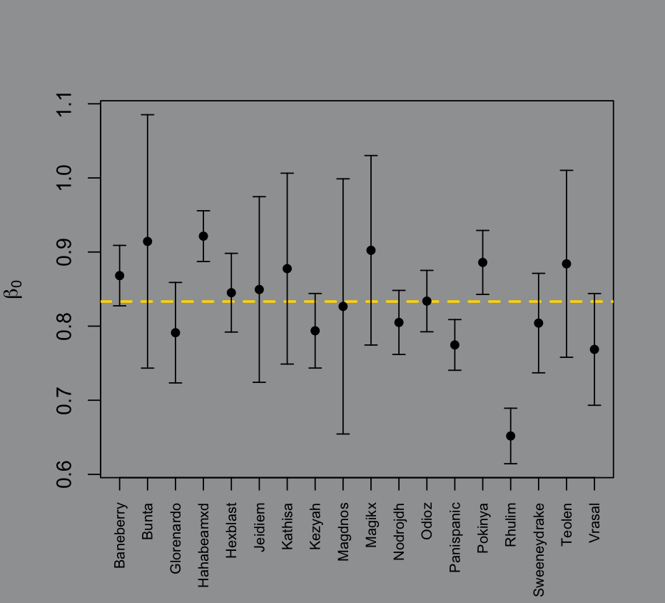

$\beta_0$ exists but in this context I don’t think it really means much. It’s the baseline of the raider’s damage prevention at pull 0, which is a little silly, but maybe someone else can extract some value from it.

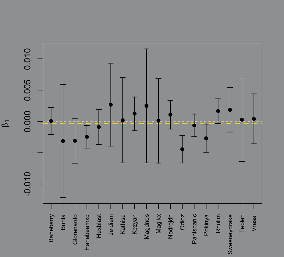
$\beta_1$ is far more interesting. It’s the trend in raider performance over every pull. A raider who gets worse over time has a negative $\beta_1$. If it’s positive they get better over time. The larger the confidence bands the more variation in their performance. So the “ideal” raider would have a $\beta_1 = 0$ with no confidence bands; they’re perfectly consistent from beginning to end.

The way that I calculated the $z$-scores for damage reduced used the global mean and standard deviation for the raid across all pulls. That’s probably not the best measurement since some roles and classes will always take and reduce higher magnitudes of damage.

I took the mean of each raider’s $z$-score and plotted it on a scatter plot:

1
# raider average z-score of damage reduced
2
z_Dr_bar = rowMeans(z_Dr)
3

4
# plot of those z-scores per raider
5
plot(seq_along(z_Dr_bar),z_Dr_bar,
6
     xaxt = "n", xlab = "", ylab = TeX("$z_{Dr}$"), type = "n")
7
# 0 line for reference
8
abline(h = 0, lty = 3, lwd = 2, col = "grey80")
9
# points layer
10
points(seq_along(z_Dr_bar), z_Dr_bar, pch = 16)
11
# raider names of the x axis
12
axis(1, seq_along(rownames(tot_dr)), rownames(tot_dr), las = 2, cex.axis = 0.7)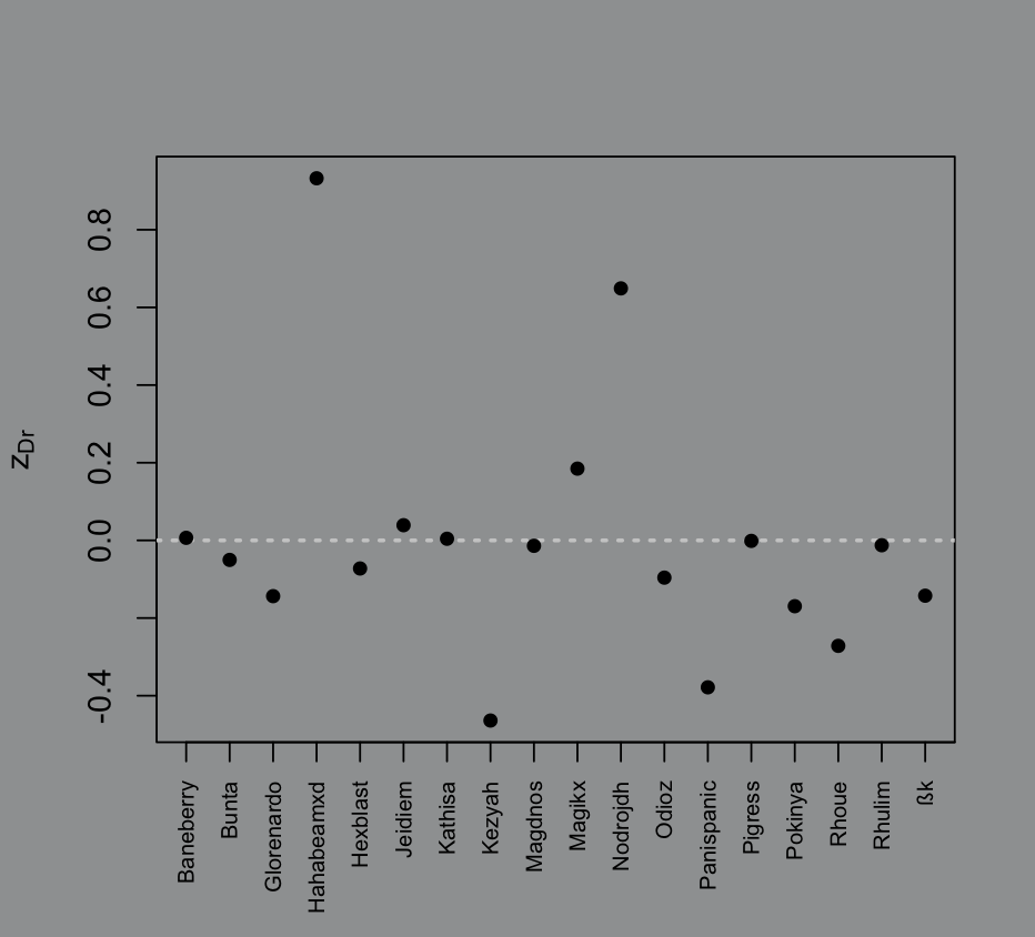

Computing a $z$-score is typically referred to as “standardizing the data” because it converts data into a standard normal distribution (given that the data was already normal).

Hypothetically, every raider should have a mean $z$-score of $\approx 0$. If someone has a higher score than they’re typically reducing more damage than the rest of the raid, vice versa if they have a lower score.

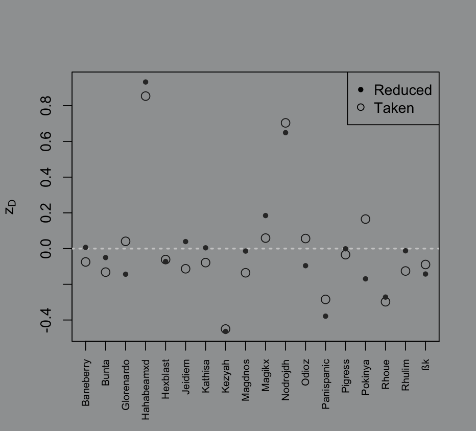
Again, this measurement isn’t the best because its basis is flawed. I also can’t work with a $z$-score for proportions because the denominator doesn’t play nice, so we’re stuck with the general issues of this $z_{Dr}$ metric. What I can do instead is calculate each set of $z$-scores for damage reduced and damage taken, then plot both values on a scatterplot. I’ll make the points for damage taken hollow and keep the points for damage reduced as is to avoid missing an overlap. Hopefully that gives more context to certain points being very high or very low.

1
# raider average z-score of damage taken
2
z_Dt_bar = rowMeans(z_Dt)
3

4
par(bg="#9EA0A1")
5
# plot of those z-scores per raider
6
plot(seq_along(z_Dt_bar),z_Dt_bar,
7
     ylim = c(min(z_Dr_bar,z_Dt_bar),max(z_Dr_bar,z_Dt_bar)),
8
     xaxt = "n", xlab = "", ylab = TeX("$z_{Dt}$"), type = "n")
9
# 0 line for reference
10
abline(h = 0, lty = 3, lwd = 2, col = "grey80")
11
# points layer, open circle for damage taken, closed for reduced
12
points(seq_along(z_Dt_bar), z_Dt_bar, cex = 1.3, col = "grey10")
13
points(seq_along(z_Dr_bar), z_Dr_bar, pch = 20, cex = 1, col = "grey20")
14
# raider names of the x axis
15
axis(1, seq_along(rownames(tot_dt)), rownames(tot_dt), las = 2, cex.axis = 0.7)
16
legend("topright", inset = c(0,0),
17
       legend = c("Reduced","Taken"),
18
       pch = c(20,1), title = "Damage")